Introduction to R Notes for Class 11 Data Science – Fully aligned with the latest CBSE syllabus and covering every important topic. Get complete, point-wise notes with clear explanations and examples, all in one place. Cover the chapter thoroughly and prepare effectively to aim for a high score in your exam. 🚀

Introduction to R Studio

• R: R is an open-source programming language widely used for statistical computing, data analysis, and data visualization.
• RStudio: RStudio is an Integrated Development Environment (IDE) used to write and execute R programs. It provides an interface for coding, viewing results, and working with data.
• RStudio allows users to load CSV files and view their contents for data analysis.
• RStudio can be installed on Windows by downloading and running its installer.

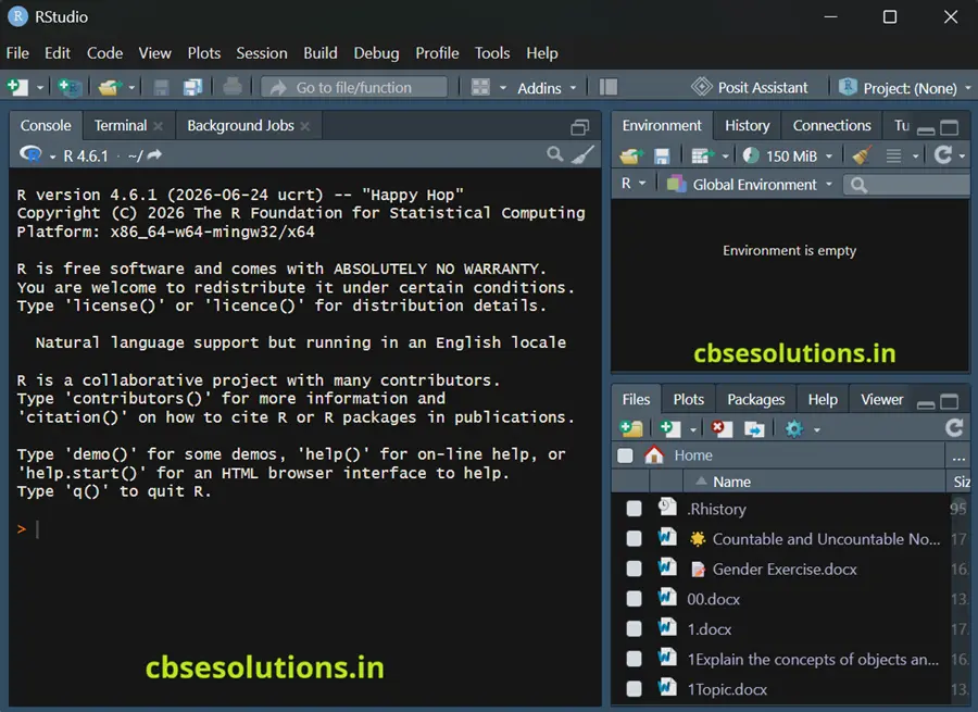
How to write and run a script

• Click the + sign below the File menu and select R Script. A new window opens on the top-left side.
• Type your code in the script window and click Run. The result appears in the Console.
• The Console is where R shows results.

RStudio Interface and Working Directory

Console: The console is the area where users can enter R commands directly and view their results. Commands entered directly into the console are not saved after closing the session.

Working Directory: The working directory is the folder where RStudio reads and saves files by default.

• getwd() function: This function displays the current working directory.
• setwd() function: This function changes the current working directory to a folder of the user’s choice. The directory path can be relative or absolute.

Example:

setwd(“C:/Users/Student/Desktop/Project”)
getwd()

Output:

# [1] “C:/Users/Student/Desktop/Project”

Vectors in R

• Vector: A vector is a sequence of elements that share the same data type. It is one of the most basic data objects in R.
• R has six basic types of atomic vectors: logical, integer, double, complex, character, and raw.
• Single-Element Vector: A vector containing only one value is called a single-element vector.
• Example:
  x <- 10
  print(x)
• Multiple-Element Vector: A vector containing more than one value is called a multiple-element vector.
• Example:
  x <- c(10, 20, 30, 40)
  print(x)

Creating a Vector

Using the Colon Operator

The colon (:) operator creates a numeric vector containing a sequence of consecutive numbers.

Example:

x <- 1:5
print(x)

Output:
1 2 3 4 5

Using the Sequence Function

The seq() function creates a sequence of numbers with a specified increment.

Example:

x <- seq(2, 10, by = 2)
print(x)

Output:
2 4 6 8 10

Using c() Function

The c() function combines multiple values into a single vector.

Example:

x <- c(10, 20, 30, 40)
print(x)

Output:
10 20 30 40

Example:

x <- c(10, 20, “Hello”)
print(x)

Output:
“10” “20” “Hello”

Vector Indexing

• Indexing is used to access individual elements of a vector.
• Square brackets ([]) are used for indexing.
• Indexing starts at position 1.

Example:

x <- c(10, 20, 30, 40)
print(x[2])

Output:
20

Negative Indexing: A negative index excludes the element at the specified position from the result.

Example:

x <- c(10, 20, 30, 40)
print(x[-2])

Output:
10 30 40

Logical Indexing: Logical values (TRUE and FALSE) can be used to select elements from a vector.

Example:

x <- c(10, 20, 30, 40)
print(x[c(TRUE, FALSE, TRUE, FALSE)])

Output: 10 30

Arithmetic Operations on Vectors

• Addition, subtraction, multiplication, and division can be performed on vectors.
• These operations are performed on corresponding elements, and the result is another vector.
• Vectors should be of same length

Example:

v1 <- c(3, 4, 5)
v2 <- c(6, 7, 8)
print(v1 + v2)
print(v1 – v2)
print(v1 * v2)
print(v1 / v2)

Output:

9 11 13
-3 -3 -3
18 28 40
0.5 0.5714 0.625

Lists in R

• A list is an R object that can store elements of different data types, such as numbers, strings, vectors, and other lists.
• It can also contain functions and matrices.

Creating a List

The list() function is used to create a list.

Example:

mylist <- list(25, “R”, TRUE, c(5, 10))
print(mylist)

Output:

[[1]]
[1] 25
[[2]]
[1] “R”
[[3]]
[1] TRUE
[[4]]
[1] 5 10

Naming and accessing list elements

• Names can be given to list elements so that they are easy to identify and access.
• An element can be accessed by its index using [ ] or by its name using $.

Example:

mylist <- list(Name = “Ravi”, Age = 17, Marks = 85)
print(mylist)
print(mylist[1]) 
print(mylist$Age)

Output:

$Name
[1] “Ravi”
$Age
[1] 17
$Marks
[1] 85

$Name  [1] “Ravi”
[1] 17

Manipulating Lists

Elements in a list can be added, deleted, or updated. Adding or deleting elements is possible only at the end of a list, whereas any element can be updated.

Example:

x <- list(10, 20, 30)
# Add an element
x <- append(x, 40)
# Update the second element
x[[2]] <- 50
# Delete the last element
x <- x[-length(x)]
print(x)

Output:
10 50 30

Merging Lists

Multiple lists can be combined into a single list using the c() or list() function.

Example:

x <- list(10, 20)
y <- list(30, 40)
z <- c(x, y)
print(z)

Output:
10 20 30 40

Converting a List into a Vector

The unlist() function converts a list into a vector. The resulting vector can be used for further operations, including arithmetic operations.

Example:

x <- list(10, 20, 30)
y <- unlist(x)
print(y)
print(y + 5)

Output:

10 20 30
15 25 35

Matrices in R

• Matrix: A matrix is a two-dimensional rectangular arrangement of elements.
• It is an extension of an atomic vector, so all its elements must have the same data type.

Creating a Matrix

The matrix() function is used to create a matrix in R.

Syntax:
matrix(data, nrow, ncol, byrow, dimnames)

• data: Specifies the input vector whose elements are used to create the matrix.
• nrow: Specifies the number of rows in the matrix.
• ncol: Specifies the number of columns in the matrix.
• byrow: Determines how elements are arranged. When set to TRUE, elements are filled row-wise. By default, they are filled column-wise.
• dimnames: Specifies the names assigned to the rows and columns.

Example:

x <- matrix(c(1, 2, 3, 4, 5, 6), nrow = 2, ncol = 3, byrow = TRUE)
print(x)

Output:
[,1] [,2] [,3]
[1,]    1    2    3
[2,]    4    5    6

Accessing Matrix Elements

Matrix elements can be accessed using their row and column indices. The syntax is matrix[row, column].

Example:

x <- matrix(1:6, nrow = 2, byrow = TRUE)
print(x[2, 3])

Output: 6

Arithmetic Operations on Matrices

Addition, subtraction, multiplication, and division can be performed on matrices of the same dimensions. The result is another matrix.

Example:

A <- matrix(c(1, 2, 3, 4), nrow = 2)
B <- matrix(c(5, 6, 7, 8), nrow = 2)
print(A + B)

Output:

[,1] [,2]
[1,]    6   10
[2,]    8   12